My R Notes
1 Uses of ggplot2
## `geom_smooth()` using method = 'loess' and formula 'y ~ x'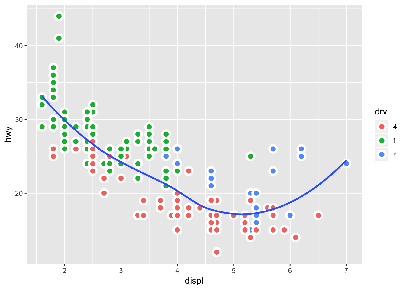
2 Data Transformations
# filter(mpg, model == "a4" & year > 2000)
# select(mpg, model:cyl)
# select(mpg, -(model:cyl))
# arrange(mpg, year, cty)
# mutate(mpg, ctyvshwy = cty - hwy)
# mutate(mpg, ctyvshwy = cty - hwy) %>% select(model, cty, hwy, ctyvshwy) %>% filter(ctyvshwy > -3)
# transmute(mpg, )
if (!require("nycflights13")) install.packages("nycflights13")
library(nycflights13)
delays <- flights %>%
group_by(dest) %>%
summarise(
count = n(),
dist = mean(distance, na.rm = TRUE),
delay = mean(arr_delay, na.rm = TRUE)
) %>%
filter(count > 20, dest != "HNL")
ggplot(delays, aes(dist, delay)) +
geom_point(aes(size = count), alpha = 1/3) +
geom_smooth(se = FALSE, span = 0.6)## `geom_smooth()` using method = 'loess' and formula 'y ~ x'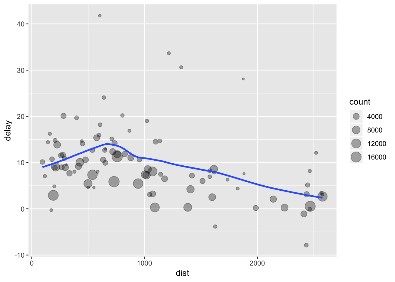
# group_by(mpg, manufacturer) %>% summarise(count = n(), mean_hwy = median(hwy, na.rm = TRUE), mean_cty = mean(cty, na.rm = TRUE), diff = mean(hwy) - mean(cty)) %>% arrange(desc(mean_hwy)) %>% filter(count %in% c(1,3,6,9) | count > 15)## `geom_smooth()` using method = 'gam' and formula 'y ~ s(x, bs = "cs")'
# var = mtcars %>% group_by(cyl) %>% summarise(count = n(), mean_mpg = mean(mpg), mean_hp = mean(hp), median_wt = median(wt))

# ggplot(var, aes(cyl,mean_mpg)) + geom_point(aes(size = mean_hp, color = median_wt))
tb <- tribble(
  ~index, ~size, ~wt,
  "1",5,10.1,
  "2",3,11.4,
  "3",2,9.98
)

tibble(
  a = lubridate::now() + runif(1e3) * 86400,
  b = lubridate::today() + runif(1e3) * 30,
  c = 1:1e3,
  d = runif(1e3),
  e = sample(letters, 1e3, replace = TRUE)
)
df <- tibble(
x = runif(5),
y = rnorm(5)
)
dfggplot(df,aes(x, y)) +
geom_point(aes(color = x))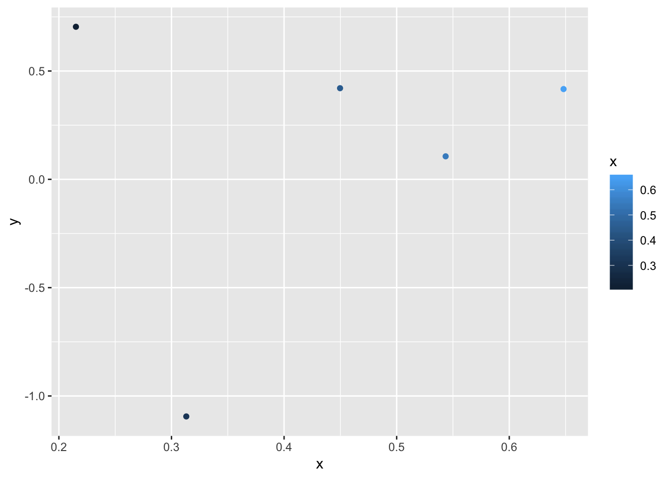
df$x## [1] 0.3131381 0.4497158 0.2151312 0.6482134 0.5434941df[["x"]]## [1] 0.3131381 0.4497158 0.2151312 0.6482134 0.5434941df[[1]]## [1] 0.3131381 0.4497158 0.2151312 0.6482134 0.5434941df %>% .$x## [1] 0.3131381 0.4497158 0.2151312 0.6482134 0.5434941df %>% .[["x"]]## [1] 0.3131381 0.4497158 0.2151312 0.6482134 0.54349413 Reading Files
read_csv("first line\n1,2,3\n4,.,6\n1,0,1", skip = 1, col_names = c("x", "y", "z"), na = ".")4 Parsing a Vector
str(parse_date(c("2010-01-01", '2019-01-01', '1990-01-01','.'), na = "."))## Date[1:4], format: "2010-01-01" "2019-01-01" "1990-01-01" NAstr(parse_character(c("a","b")))## chr [1:2] "a" "b"parse_double("1,23", locale = locale(decimal_mark = ","))## [1] 1.23parse_number(c("$100","20%","40 dollars", "#50"))## [1] 100 20 40 50charToRaw("Leriche")## [1] 4c 65 72 69 63 68 65charToRaw(".")## [1] 2et <- charToRaw("b")
rawToChar(t)## [1] "b"library(hms)
parse_time("01:10 am")## 01:10:00guess_parser("2018-10-04")## [1] "date"5 Exporting/Importing Files
# write_excel_csv()

# write_csv(data, "filename.csv")

# readxl()

# haven()  reads spss, stata and SAS files.
# gather()
table4a <- tribble(
~"country",~`1999`,~`2000`,
"USA", 444, 888,
"BRA", 232, 458
)
table4a %>%
gather(`1999`, `2000`, key = "year", value = "cases")# spread()
table2 <- tribble(
~"country",~"year",~"type",~"count",
"USA", 1999, "cases", 759,
"USA", 1999, "population", 87432,
"USA", 2000, "cases", 888,
"USA", 2000, "population", 499843
)
table2(table2 %>%
spread(key = type, value = count))# separate()
table3 <- tribble(
~"country",~"year",~"rate",
"USA", 2000, "586/58943",
"USA", 2001, "588/76633",
"FRA", 2001, "45323/12345"
)
table5 <- table3 %>%
separate(rate, into = c("cases","population"), convert = TRUE) %>%
separate(year, into = c("century", "year"), sep = 2)# unite(new, century, year)
table5 %>%
unite(new, century, year, sep = "")stocks <- tibble(
year = c(2015, 2015, 2015, 2015, 2016, 2016, 2016),
qtr = c( 1, 2, 3, 4, 2, 3, 4),
return = c(1.88, 0.59, 0.35, NA, 0.92, 0.17, 2.66)
)
stocks %>%
spread(qtr, return)stocks %>%
spread(year, return) %>%
gather(year, return, `2015`:`2016`, na.rm = TRUE)# complete()
stocks %>%
complete(year, qtr)treatment <- tribble(
~ person, ~ treatment, ~response,
"Derrick Whitmore", 1, 7,
NA, 2, 10,
NA, 3, 9,
"Katherine Burke", 1, 4
)
treatment %>%
fill(person)who1 <- who %>%
gather(new_sp_m014:newrel_f65, key = "key", value = "cases", na.rm = TRUE)
who1 %>%
count(key)who2 <- who1 %>%
mutate(key = stringr::str_replace(key, "newrel", "new_rel"))
who2who3 <- who2 %>%
separate(key,c("new","type","sexage"), sep = "_")
who3who3 %>%
count(new)who4 <- who3 %>%
select(-new, -iso2, -iso3)
who5 <- who4 %>%
separate(sexage, c("sex","age"), sep = 1)
who5planes %>%
count(tailnum) %>%
filter(n>1)weather %>%
count(year, month, day, hour, origin) %>%
filter(n>1)flights2 <- flights %>%
select(year:day, hour, origin, dest, tailnum, carrier)
flights2 flights2 %>%
select(-origin, -dest) %>%
left_join(airlines, by = "carrier")flights2 %>%
select(-origin, -dest) %>%
mutate(name = airlines$name[match(carrier, airlines$carrier)])flights2 %>%
left_join(airports, c("dest" = "faa")) %>%
arrange(origin)flights2 %>%
left_join(airports, c("origin" = "faa")) %>%
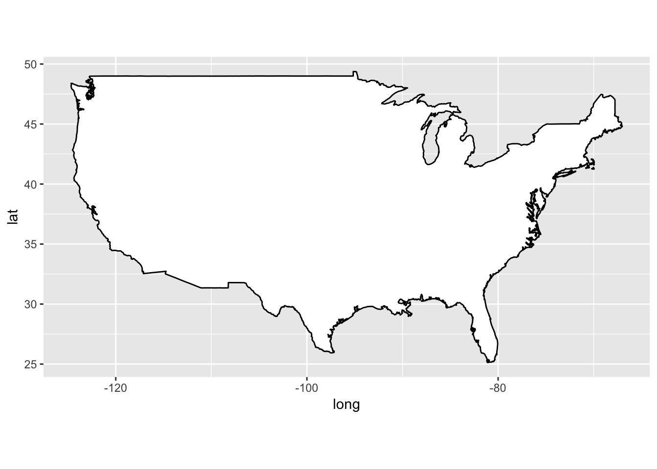
arrange(origin)airports %>%
semi_join(flights, c("faa" = "dest")) %>%
filter(lon > -140) %>%
ggplot(aes(lon, lat)) +
borders("state") +
geom_point(aes(color = alt)) +
coord_quickmap()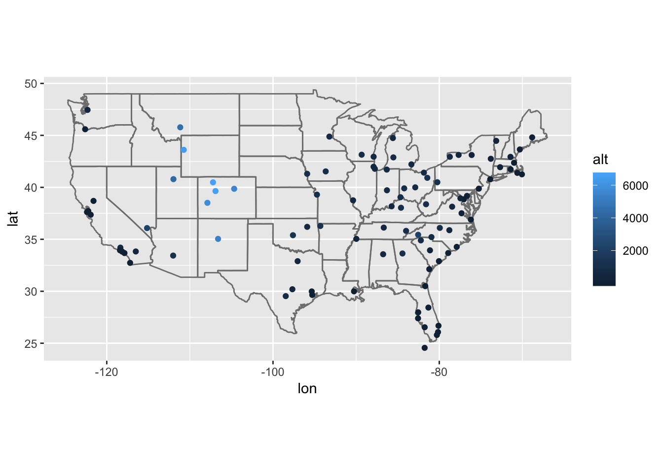
(top_dest <- flights %>%
  count(dest, sort = TRUE) %>%
  head(10))
top_dest <- flights %>%
count(dest, sort = TRUE) %>%
left_join(airports, c("dest" = "faa"))
top_destflights %>%
filter(dest %in% top_dest$dest)6 Strings
x <- "\u00b5"
x
## [1] "µ"string <- c("x","y","z")
string## [1] "x" "y" "z"str_c("x","y","z")## [1] "xyz"str_c("x","y","z", sep = ", ")## [1] "x, y, z"name <- "Tomas"
time_of_day <- "morning"
birthday <- FALSE
str_c(
"Good ", time_of_day, " ", name,
if (birthday) " and HAPPY BIRTHDAY",
"."
)## [1] "Good morning Tomas."str_c(c("x", "y", "z"), collapse = ":")## [1] "x:y:z"x <- c("Apple", "Banana", "Pear")
str_sub(x, 1, 2)## [1] "Ap" "Ba" "Pe"str_sub(x, -3, -1)## [1] "ple" "ana" "ear"str_sub(x, 1, 1) <- str_to_lower(str_sub(x, 1, 1))
x## [1] "apple" "banana" "pear"x <- c("x","d","y","u","q","a","b")
str_sort(x)## [1] "a" "b" "d" "q" "u" "x" "y"x <- c("xylophone","apples","pears","chicken","pork","ate","bee")
str_view(x, "a")7 Determine Matches
writeLines(x)## xylophone
## apples
## pears
## chicken
## pork
## ate
## beestr_detect(x, "e")## [1] TRUE TRUE TRUE TRUE FALSE TRUE TRUEsum(str_detect(words, "[aeiou]$"))## [1] 271mean(str_detect(words, "[aeiou]$"))## [1] 0.2765306no_vowels_1 <- !str_detect(words, "[aeiou]")
no_vowels_2 <- str_detect(words, "^[^aeiou]+$")
identical(no_vowels_1, no_vowels_2)## [1] TRUE8 Models
if (!require("modelr")) install.packages("modelr")
library(modelr)
options(na.action = na.warn)

ggplot(sim1, aes(x, y)) +
  geom_point()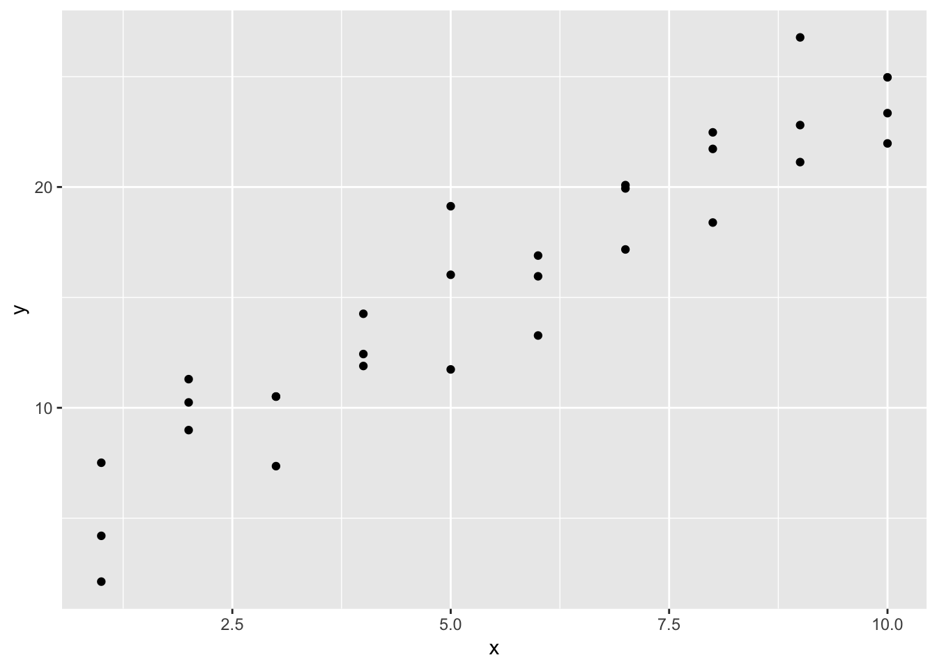
models <- tibble(
  a1 = runif(250, -20, 40),
  a2 = runif(250, -5, 5)
)

ggplot(sim1,aes(x,y)) +
  geom_abline(aes(intercept=a1,slope=a2), models, alpha = 1/4) +
  geom_point()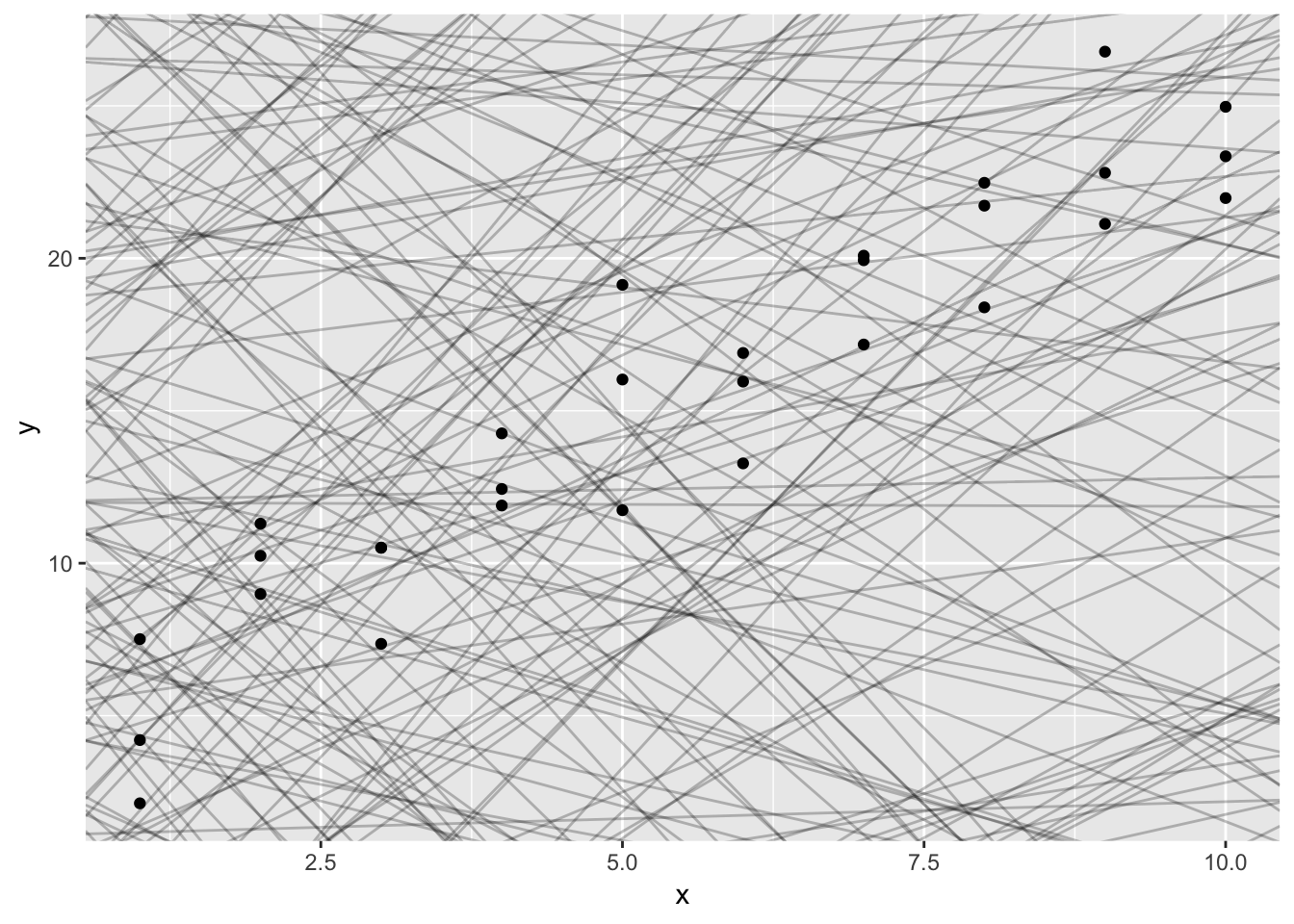
model1 <- function(a, data) {
  a[1] + data$x * a[2]
}

model1(c(5,5), sim1)
## [1] 10 10 10 15 15 15 20 20 20 25 25 25 30 30 30 35 35 35 40 40 40 45 45
## [24] 45 50 50 50 55 55 559 Root-mean-squared deviation
measure_dist <- function(mod, data) {
  diff <- data$y - model1(mod, data)
  diff^2 %>%
    mean() %>%
    sqrt()
}
measure_dist(c(5,5), sim1)
## [1] 19.1077410 Fitting linear models with lm()
sim1_mod <- lm(y ~ x, data = sim1)

coef(sim1_mod)
## (Intercept) x
## 4.220822 2.051533sim1a <- tibble(
x = rep(1:10, each = 3),
y = x * 1.5 + 6 + rt(length(x), df = 2)
)
sim1a_mod <- lm(y ~ x, data = sim1a)
coef(sim1a_mod)## (Intercept) x
## 5.694273 1.639591grid <- sim1 %>%
data_grid(x)
gridgrid <- grid %>%
add_predictions(sim1_mod)
grid11 Prime Find Func
primary <- function(x) {
  if (min(x %% 2:(x-1)) > 0) {
    return(x)
  }else{
    return(0)
  }
}

array = c(1:1000)

primeArray <- matrix()

count = 0

for (x in array) {
  if (x == 1) {
    next
  }
  if (primary(x) > 0) {
    primeArray <- append(primeArray, x)
    count = count + 1
  }

}
primeArray <- primeArray[!is.na(primeArray)]
count
## [1] 167primeArray## [1] 3 5 7 11 13 17 19 23 29 31 37 41 43 47 53 59 61
## [18] 67 71 73 79 83 89 97 101 103 107 109 113 127 131 137 139 149
## [35] 151 157 163 167 173 179 181 191 193 197 199 211 223 227 229 233 239
## [52] 241 251 257 263 269 271 277 281 283 293 307 311 313 317 331 337 347
## [69] 349 353 359 367 373 379 383 389 397 401 409 419 421 431 433 439 443
## [86] 449 457 461 463 467 479 487 491 499 503 509 521 523 541 547 557 563
## [103] 569 571 577 587 593 599 601 607 613 617 619 631 641 643 647 653 659
## [120] 661 673 677 683 691 701 709 719 727 733 739 743 751 757 761 769 773
## [137] 787 797 809 811 821 823 827 829 839 853 857 859 863 877 881 883 887
## [154] 907 911 919 929 937 941 947 953 967 971 977 983 991 99712 Order()
v <- c(12, 11, 5, 22, 5)

b <- c("abc", "bcv", "aab")

order(v)
## [1] 3 5 2 1 4v <- v[order(v)]
v## [1] 5 5 11 12 22b <- b[order(b)]
b## [1] "aab" "abc" "bcv"a <- c(1,4,2,3)
order(a)## [1] 1 3 4 213 Lists()
a <- matrix(1:6, nrow = 2, byrow = TRUE)


c <- list("a" = a, "b" = 5:7)

c
## $a
## [,1] [,2] [,3]
## [1,] 1 2 3
## [2,] 4 5 6
##
## $b
## [1] 5 6 7c$b[2]## [1] 6c[["b"]][[2]]## [1] 6d <- list("e" = c, "f" = c)
d## $e
## $e$a
## [,1] [,2] [,3]
## [1,] 1 2 3
## [2,] 4 5 6
##
## $e$b
## [1] 5 6 7
##
##
## $f
## $f$a
## [,1] [,2] [,3]
## [1,] 1 2 3
## [2,] 4 5 6
##
## $f$b
## [1] 5 6 7Copyright © 2019 Tomas Leriche. All rights reserved.