Kaggle Data Analysis

This is an R Markdown notebook. I’m using this to demonstrate using R and R Notebooks. The Example is based on the Exploring Kaggle Data Science Survery from DataCamp.

dim(data)

## [1] 16716   228

data <- as.data.frame(data)

data %>%
  group_by(MLMethodNextYearSelect) %>%
  summarize(count = n()) %>%
  arrange(desc(count)) %>%
  top_n(9) %>%
  filter(!is.na(MLMethodNextYearSelect)) %>%
  
  ggplot(aes(reorder(MLMethodNextYearSelect,count), count, fill = MLMethodNextYearSelect)) +
  geom_col() +
  coord_flip() +
  scale_fill_brewer(palette = "Set2") +
  theme_bw() +
  theme(legend.position = "none") +
  xlab("ML Tool Next Year")

## Selecting by count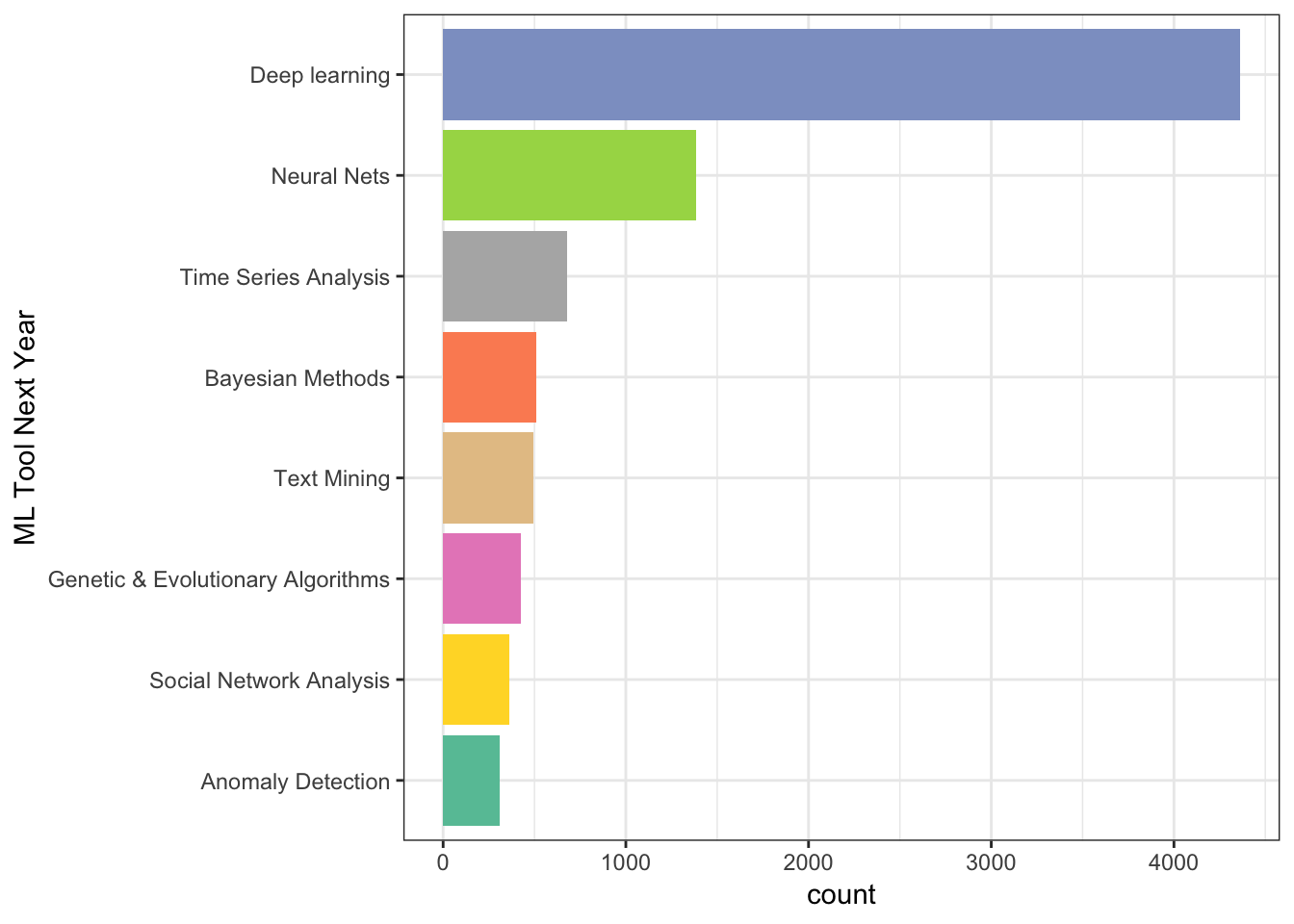

data %>%
  group_by(MLToolNextYearSelect) %>%
  summarize(count = n()) %>%
  arrange(desc(count)) %>%
  top_n(9) %>%
  filter(!is.na(MLToolNextYearSelect)) %>%
  
  
  ggplot(aes(reorder(MLToolNextYearSelect,count), count, fill = MLToolNextYearSelect)) +
  geom_col() +
  coord_flip() +
  scale_fill_brewer(palette = "Set2") +
  theme_bw() +
  theme(legend.position = "none") +
  xlab("ML Tool Next Year")

## Selecting by count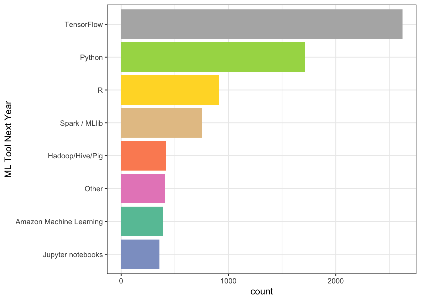

typeof(data)

## [1] "list"

df <- data %>%
  group_by(FormalEducation, GenderSelect) %>%
  filter(GenderSelect == "Male" | GenderSelect == "Female") %>%
  summarise(count = n())
  
edutotal <- df %>%
  group_by(FormalEducation) %>%
  summarise(total = sum(count))

df <- inner_join(df, edutotal, by = 'FormalEducation')

df <- df %>%
  group_by(FormalEducation, GenderSelect) %>%
  summarize(prop = count/total) %>%
  arrange(prop) %>%
  
  ggplot(aes(reorder(FormalEducation,prop), prop, fill = GenderSelect)) +
    geom_col(position = "dodge") +
    coord_flip(ylim=c(0,1)) +
    theme(legend.position="none") +
    xlab("") + 
    ggtitle("Men/Women") +
    scale_y_continuous(expand = c(0, 0)) +
    theme(axis.text.x = element_text(angle=0,
                                    vjust=0,
                                    hjust=0))
    
  
df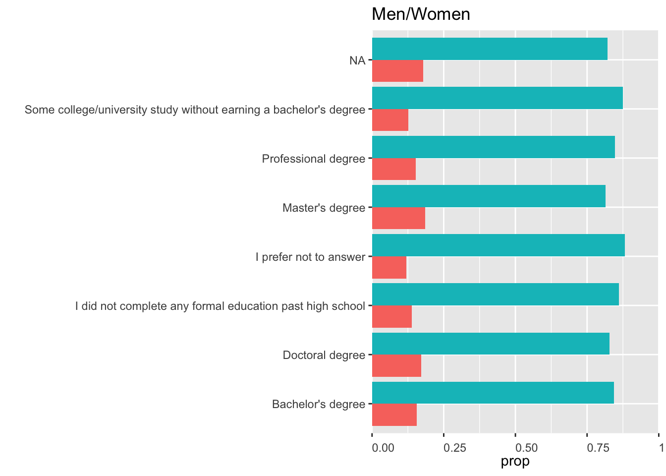

# Data Exploration

df <- data %>%
  group_by(FormalEducation, GenderSelect) %>%
  filter(GenderSelect == "Male" | GenderSelect == "Female") %>%
  summarise(count = n())
ggplot(df,aes(GenderSelect, count)) + geom_col(aes(fill = FormalEducation))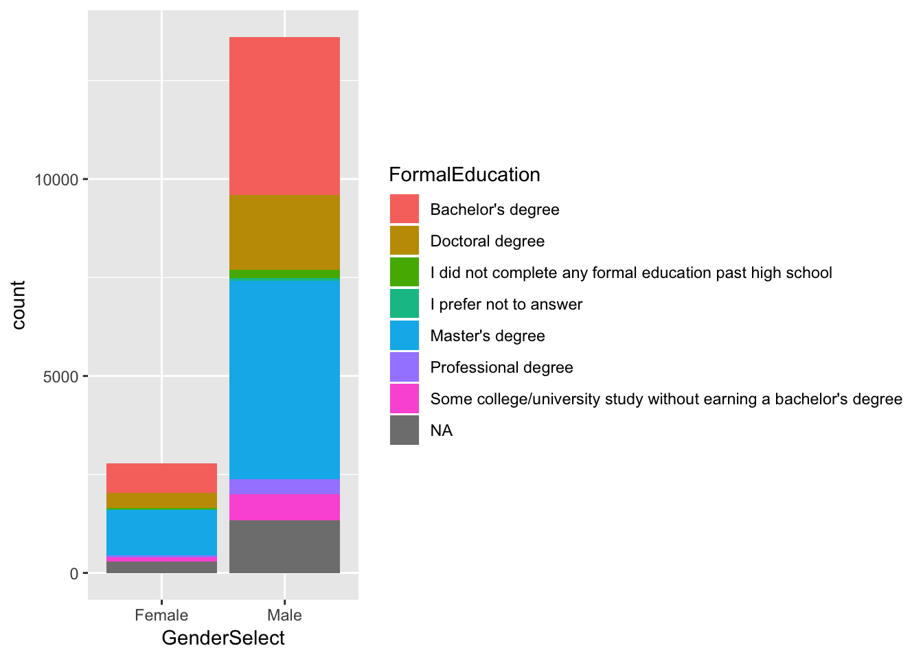

data %>%
  group_by(GenderSelect, StudentStatus) %>%
  filter(GenderSelect == "Female" | GenderSelect == "Male") %>%
  summarize(count = n())

data %>% group_by(LearningPlatformSelect) %>%
  summarise(count = n())

learning <- data
respondent <- 1:nrow(learning)

learning <- cbind(respondent, learning)


learning <- learning %>%
  select(respondent, GenderSelect, Country, Age, EmploymentStatus, LearningPlatformSelect) %>%
  mutate(learntools = strsplit(LearningPlatformSelect, split = ",")) %>%
  unnest()


learning <- learning  %>% 
    group_by(learntools)  %>% 
    summarise(numres = n())

learning <- learning %>%
  filter(numres > 1000) %>%
  arrange(desc(numres)) %>%
  filter(!is.na(learntools)) 
  
  
ggplot(learning, aes(reorder(learntools, numres), numres, fill = learntools)) +    
    geom_col() +
    coord_flip() +
    theme(legend.position="none") +
    xlab("Learning Tool") +
    ylab("Count")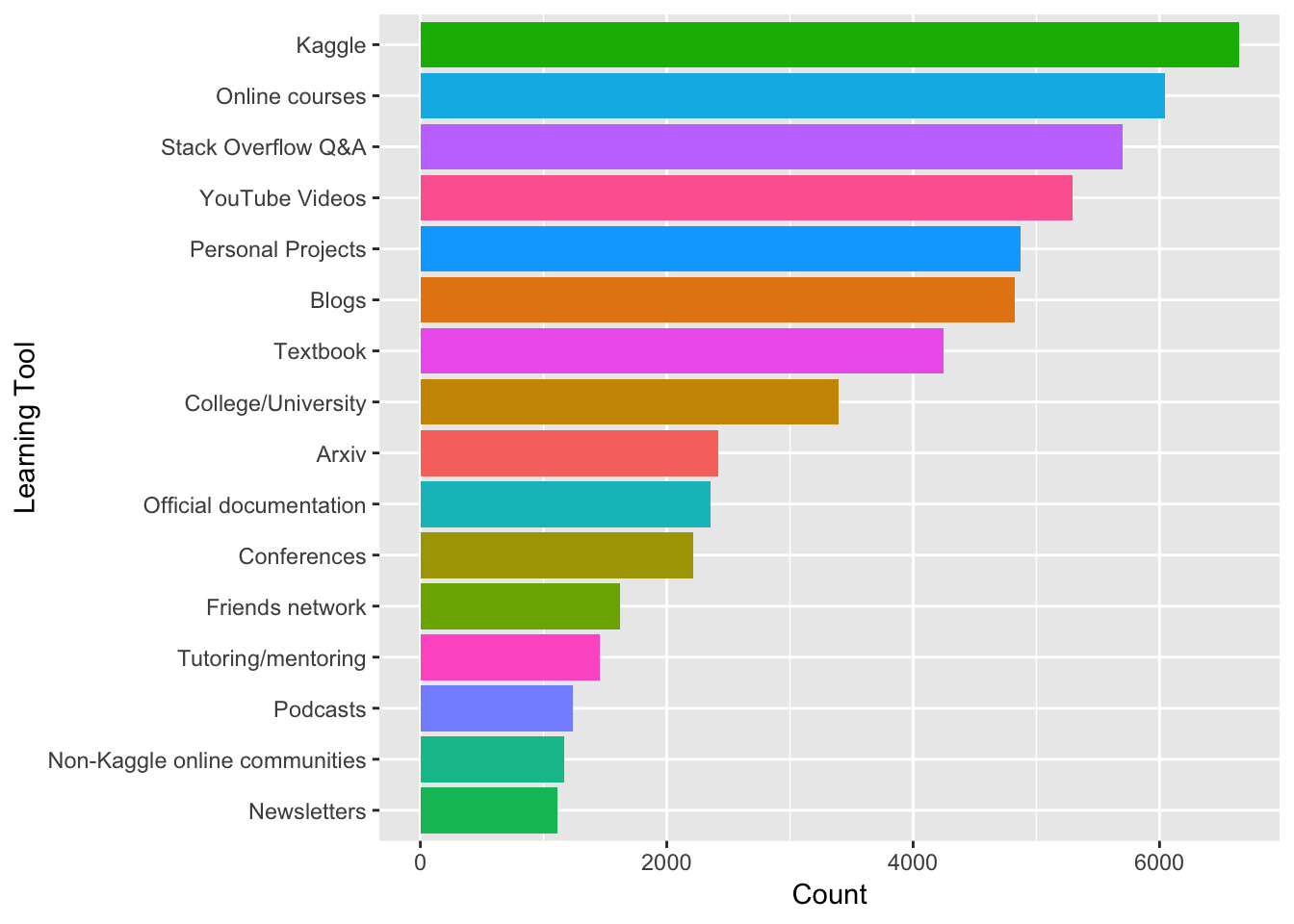

unique(data$LearningDataScienceTime)

## [1] NA            "1-2 years"   "< 1 year"    "3-5 years"   "15+ years"  
## [6] "5-10 years"  "10-15 years"

df <- data %>%
  group_by(LearningDataScienceTime, GenderSelect) %>%
  summarise(count = n()) %>%
  arrange(LearningDataScienceTime) %>%
  filter(GenderSelect == "Male" | GenderSelect == "Female") %>%
  filter(!is.na(LearningDataScienceTime))

ggplot(df,aes(reorder(LearningDataScienceTime,count), count, fill = GenderSelect)) +
  geom_col(position = "dodge") +
  coord_flip()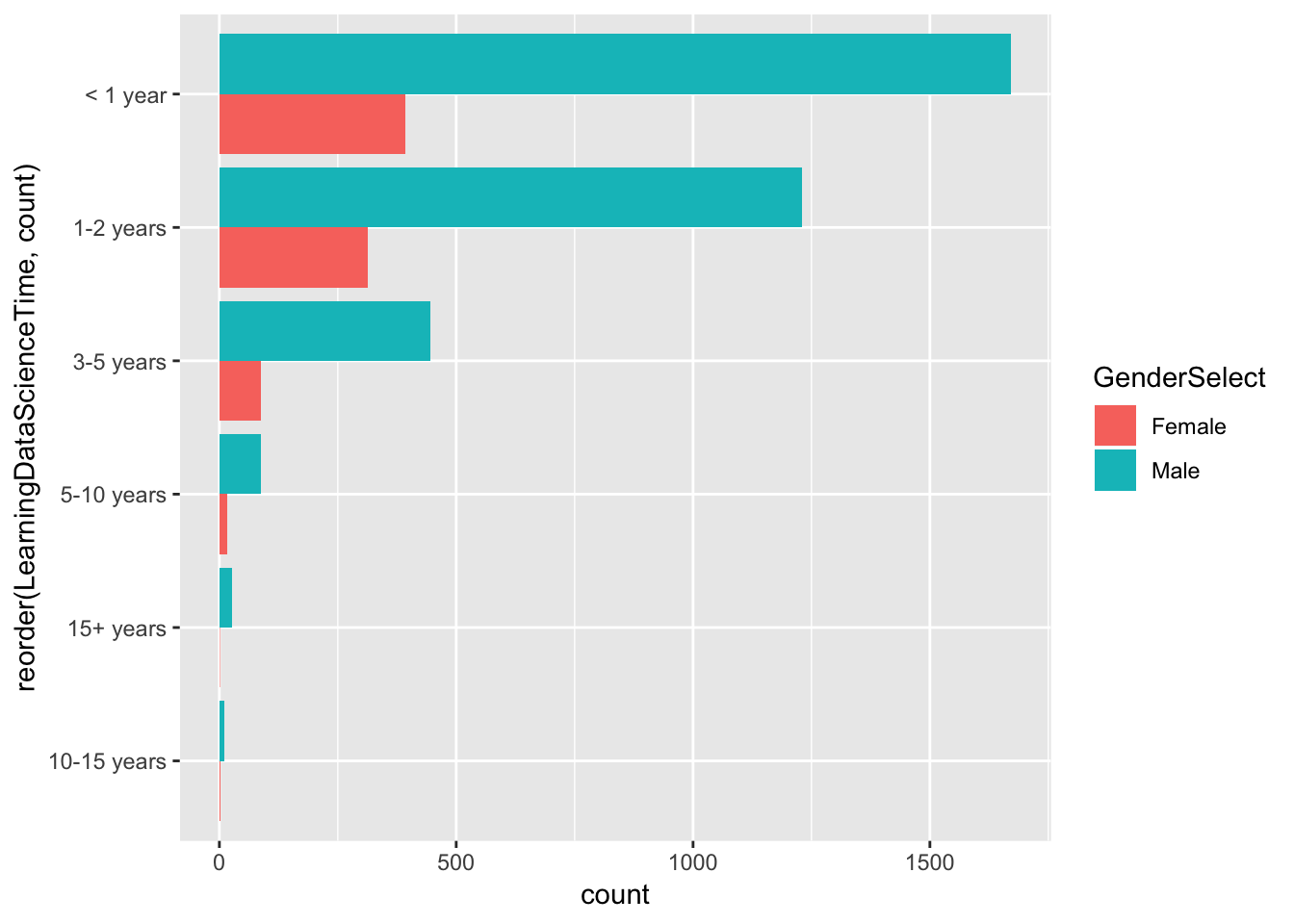

df <- df %>% group_by(LearningDataScienceTime) %>%
  mutate(total = sum(count))

df <- df %>% 
  mutate(prop = count/mean(total))

df$LearningDataScienceTime <- as.factor(df$LearningDataScienceTime)

df %>%
  ggplot(aes(LearningDataScienceTime, prop, fill = GenderSelect)) +
  geom_col(position = "dodge")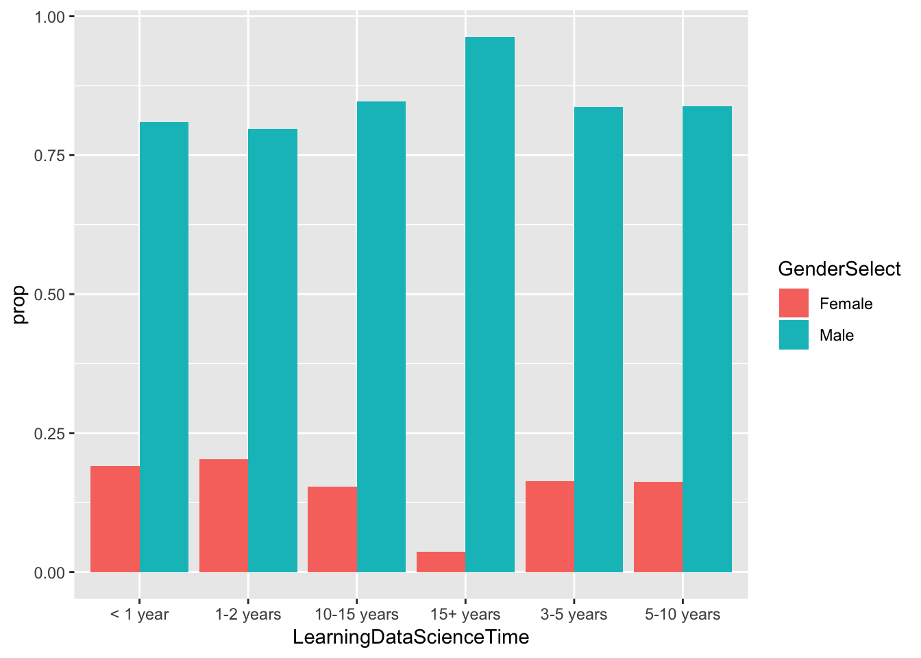

name <- function(variables) {
  
  
}

df <- data %>%
  group_by(LanguageRecommendationSelect) %>%
  summarise(count = n()) %>%
  filter(count > 90)
  
df <- df[complete.cases(df), ]

ggplot(df,aes(LanguageRecommendationSelect, count)) + geom_col(aes(fill = LanguageRecommendationSelect)) + scale_y_continuous(expand = c(0,0)) +
  theme(legend.position="none") +
  coord_flip()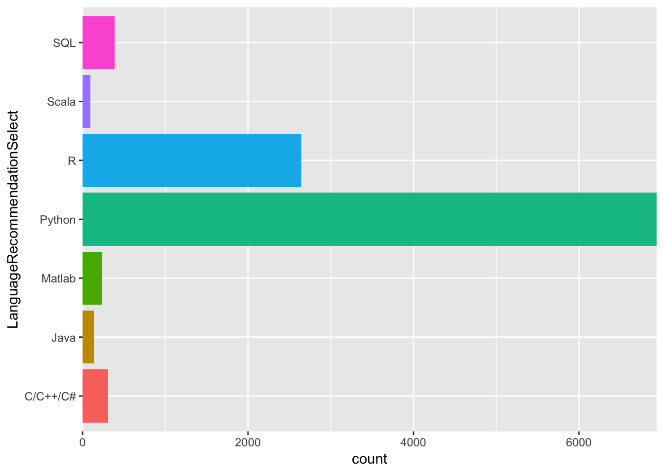

df <- data

df <- df[c("LanguageRecommendationSelect","Age", "GenderSelect")]

df <- df[complete.cases(df), ]

df <- df %>%
  mutate(Age = floor(Age/10) * 10)

df <- df %>% group_by(Age, LanguageRecommendationSelect) %>%
  summarise(count = n()) %>%
  filter(LanguageRecommendationSelect == "R" | LanguageRecommendationSelect == "Python")

df %>% ggplot(aes(Age, count, fill = LanguageRecommendationSelect)) + geom_col(position = position_dodge())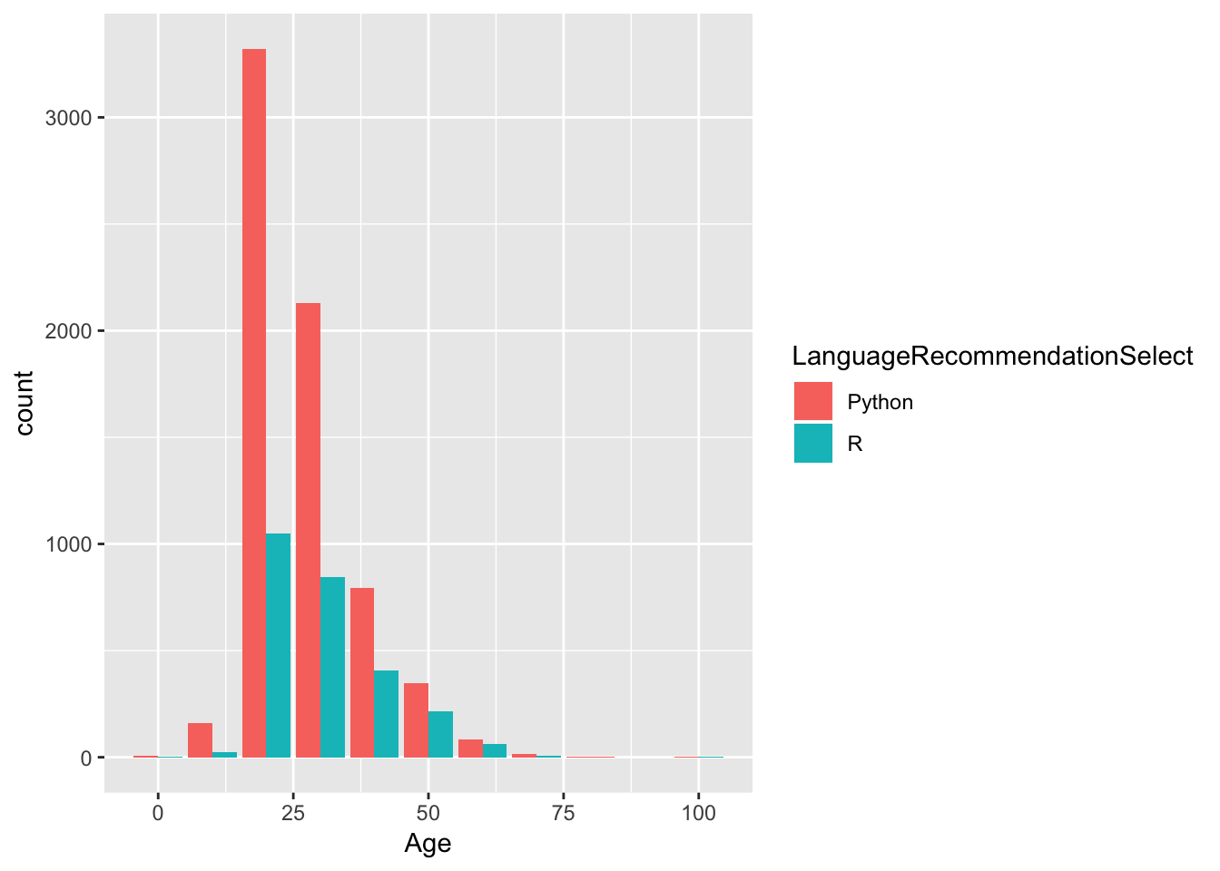

0.1 Split and Unnest()

tools <- tools %>%
  mutate(worktools = strsplit(WorkToolsSelect, split = ",")) %>%
  unnest()

tools %>% select(Respondent ,worktools)

0.2 Most Popular Language

library(RColorBrewer)
tools_count <- tools

# group by work_tools and show counts
tools_count <- tools_count  %>% 
    group_by(worktools)  %>% 
    summarise(numres = n())

tools_count <- tools_count %>%
  filter(numres > 1000) %>%
  arrange(desc(numres))
  
  
ggplot(tools_count, aes(reorder(worktools, numres), numres, fill = worktools)) +    
    geom_col() +
    coord_flip() +
    theme(legend.position="none")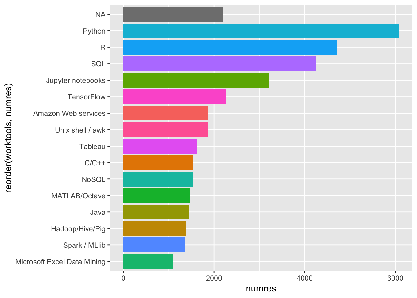

  #theme(axis.text.x = element_text(angle=20,
  #                                  vjust=0.5,
  #                                  hjust=1))

0.3 Pie Chart

pie_tools <- tools_count
pie_tools <- pie_tools %>% filter(numres > 2000)

pie_tools %>% 
  ggplot(aes("", numres, fill = worktools)) +
  geom_bar(width = 1, stat = "identity") +
  coord_polar("y", start=0) + 
  theme(axis.text.x=element_blank())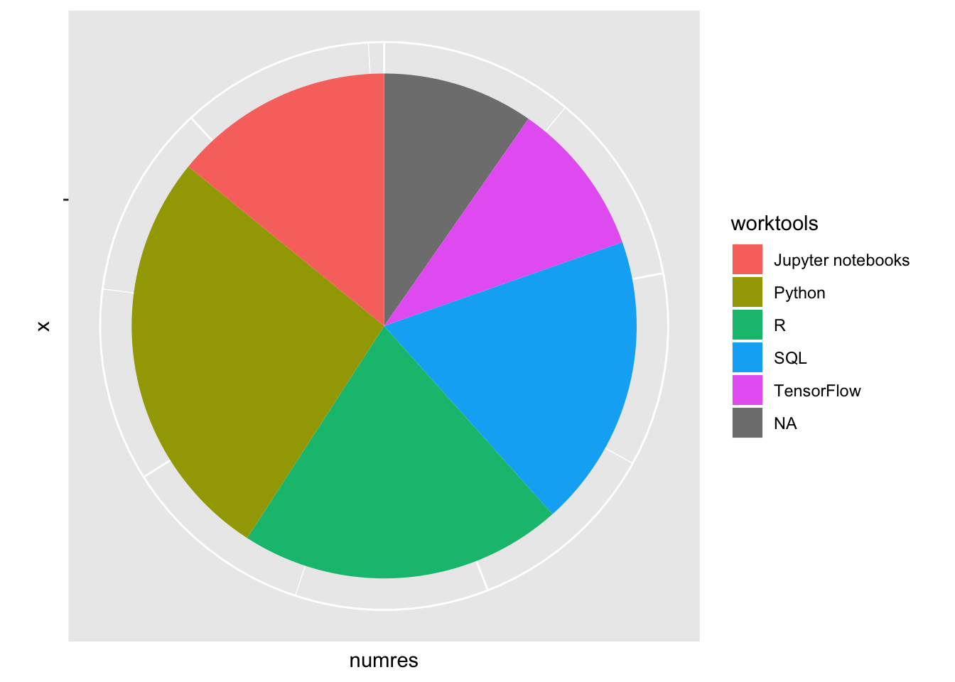

0.4 People Using R, Python, or Both

debate_tools <- df

# Creating a new column called language preference
debate_tools <- debate_tools  %>% 
   mutate(language_preference = case_when(grepl("R", WorkToolsSelect) & ! grepl("Python", WorkToolsSelect) ~ "R",
                                         grepl("Python", WorkToolsSelect) & ! grepl("R", WorkToolsSelect) ~ "Python",
                                         grepl("R", WorkToolsSelect) & grepl("Python", WorkToolsSelect) ~ "Both"))

rp_battle <- debate_tools %>% 
  group_by(language_preference) %>%
  summarize(count = n())

rp_battle

rp_battle <- rp_battle[complete.cases(rp_battle), ]
# or you could use 
#rp_battle <- filter(rp_battle, !is.na(language_preference))

rp_battle %>% ggplot(aes(language_preference, count, fill = language_preference)) + geom_col() + coord_flip() +
  scale_fill_brewer(palette = "Set2") +
  theme_bw() +
  theme(legend.position = "none")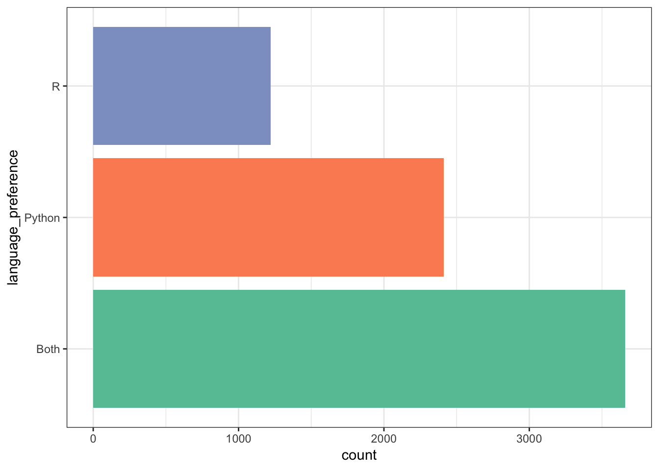

0.5 Who Recommends What?

recommendations <- debate_tools
debate_tools  <- debate_tools %>% filter(!is.na(LanguageRecommendationSelect))

recommendations <- recommendations  %>% 
    group_by(language_preference, LanguageRecommendationSelect)  %>% 
    summarize(count = n())


recommendations <- recommendations %>% arrange(desc(count)) %>%
  mutate(rank = row_number()) %>%
  filter(rank <= 4)  %>%
  arrange(language_preference)

0.6 Facet_wrap Plot

ggplot(recommendations, aes(LanguageRecommendationSelect, count, fill = LanguageRecommendationSelect)) +
  geom_bar(stat = "identity") +
  facet_wrap(~ rank, scales = "free_y") +
  scale_fill_brewer(palette = "Set2") +
  theme_bw() +
  theme(legend.position = "none") + 
  ggtitle("rank")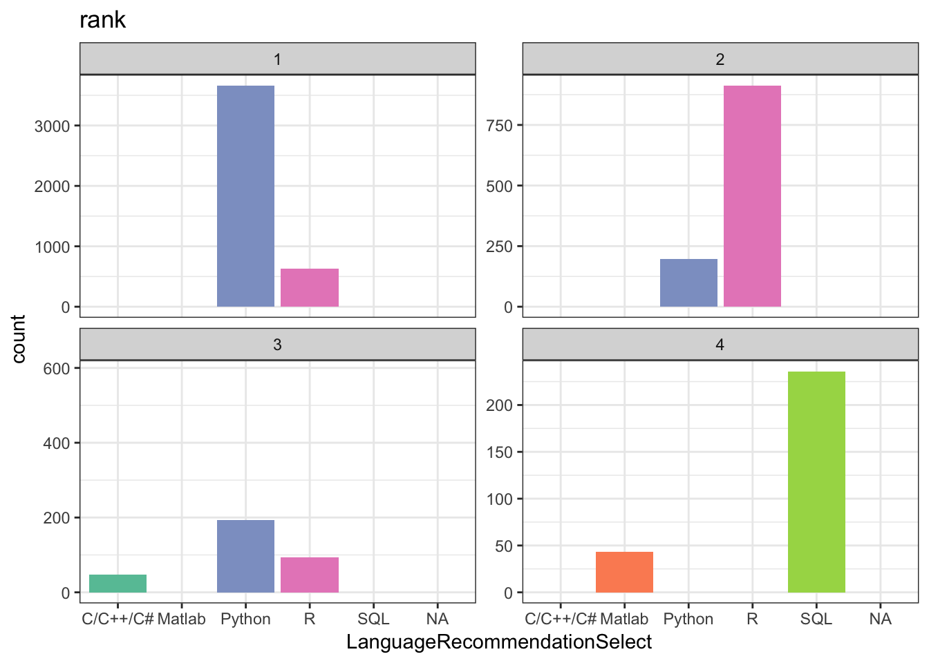

0.7 Summation

It looks like python is the clear winner by popularity, but R isn’t too far behind.