1 Text Analysis
Some of my favorite areas of data analysis are text mining and sentiment analysis. I included work I did for an assignemnt in a graduate level course I took during my Master’s (basically ch.2 material of Text Mining with R). We would eventually work through the entire book and we also conducted the analysis using SAS. I also included some other examples.
#if (!require("devtools")) install.packages("devtools")
#install.packages("devtools")

#devtools::install_github("josiahparry/geniusR")
2 Read Data
Goal: Identify product aspects in a review and classify their sentiments.
if (!require("readxl")) install.packages("readxl")
if (!require("tidytext")) install.packages("tidytext")
if (!require("dplyr")) install.packages("dplyr")
if (!require("ggplot2")) install.packages("ggplot2")
if (!require("stringr")) install.packages("stringr")
if (!require("tidyr")) install.packages("tidyr")
# first we import our data file

library(readxl)
# this path will work as long as the data.xlsx is in the same directory as this markdown file.
commentData = read_excel("./data.xlsx")

if (!require("tibble")) install.packages("tibble")
library(tibble)
#this gets us the comments for each of the 6 reviews (3 good, 3 bad)
textData = commentData[,1:10]
# here I add a column to number the reviews.
textDatalibrary(tidytext)
# here we can see the sentiments by word and lexicon 27,314 rows
sentiments# there are 4 general-purpose lexicons to choose from.
# AFINN
# bing
# nrc
# and loughran
get_sentiments("afinn")get_sentiments("bing")get_sentiments("nrc")get_sentiments("loughran")#unnest_tokens makes it so that there is one-token-per-document-per-row
tokenizedData = unnest_tokens(textData, word, text)
# 1.8 million rows
tokenizedData3 Remove Stop Words
library(dplyr)


tidyData = tokenizedData %>%
  anti_join(stop_words, by = 'word')

tidyData
# 734,4624 Count Words from Reviews
Here we count the words from all reviews We then count the words and sort by most frequent to least.
tidyData %>%
  count(word, sort = TRUE)
# we can see that br is the most frequent word.....
# examining the data we can see this is because it was collected by a web scrapper
# and it included the <br /> which designates a new line in HTML5 Plotting with ggplot2
library(ggplot2)
# the plot is ignoring the br word and showing frequencies above 1,100
tidyData %>%
  count(word, sort = TRUE) %>%
  filter(n > 1100 & n < 20000) %>%
  mutate(word = reorder(word, n)) %>%
  ggplot(aes(word, n)) +
  geom_col() +
  xlab(NULL) +
  coord_flip()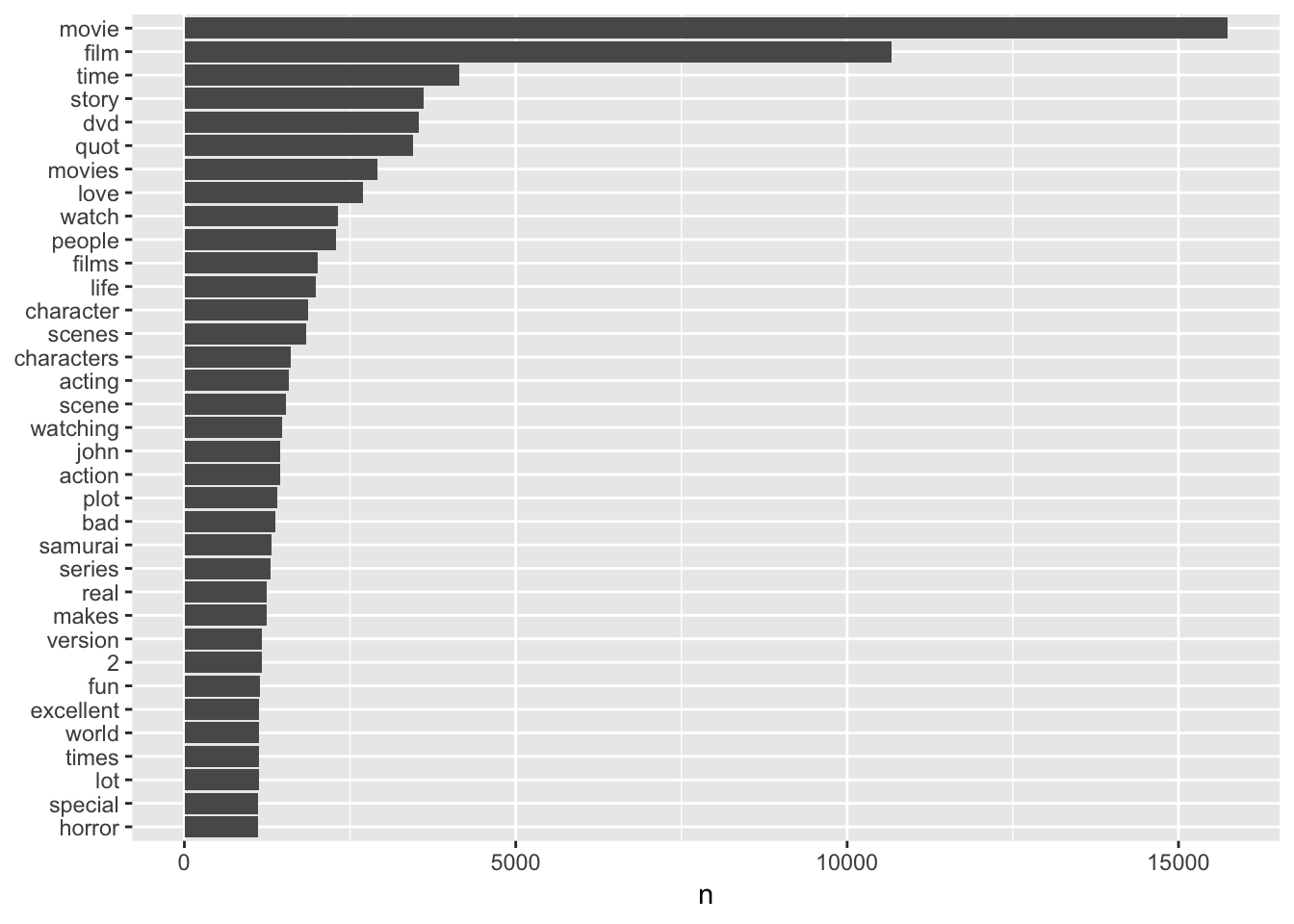
6 Sentiment Analysis
library(stringr)
# lets count 'joy' words in the reviews

nrc_joy = get_sentiments("nrc") %>%
  filter(sentiment == "joy")

# the joy words from the nrc lexicon


# here I savee the -4 afinn lexicon words to inner join later
afinn = get_sentiments("afinn") %>%
  filter(score == -4)

# here we can filter where we count the joy words by filtering for score

tidyData %>%
  filter(score == 1) %>%
  inner_join(nrc_joy, by = "word") %>%
  count(word, sort = TRUE)
# here we notice that five star rating have more joy words
tidyData %>%
filter(score == 5) %>%
inner_join(nrc_joy, by = "word") %>%
count(word, sort = TRUE)#interestingly we can see that the 5 star reviews use more or the negative words
# from the afinn lexicon than 1 star reviews.
tidyData %>%
filter(score == 5) %>%
inner_join(afinn, by = "word") %>%
count(word, sort = TRUE)tidyData %>%
filter(score == 1) %>%
inner_join(afinn, by = "word") %>%
count(word, sort = TRUE)7 Plotting
library(tidyr)
library(ggplot2)

review_sentiments = tidyData %>%
  inner_join(get_sentiments("bing"), by = "word") %>%
  count(score, sentiment) %>%
  spread(sentiment, n, fill =0) %>%
  mutate(sentiment = positive - negative)


# here I plot the data of the 111,111 reviews and group them by score, we can see that
# the scores almost perfectly match an increasing amount of positive word values
# here, for each reveiw, the negative words score count were removed form the positive
# words score count. we notice that score of 5 did indeed have majority positive words.

ggplot(review_sentiments,aes(score, sentiment, fill = score)) +
  geom_col(show.legend = FALSE)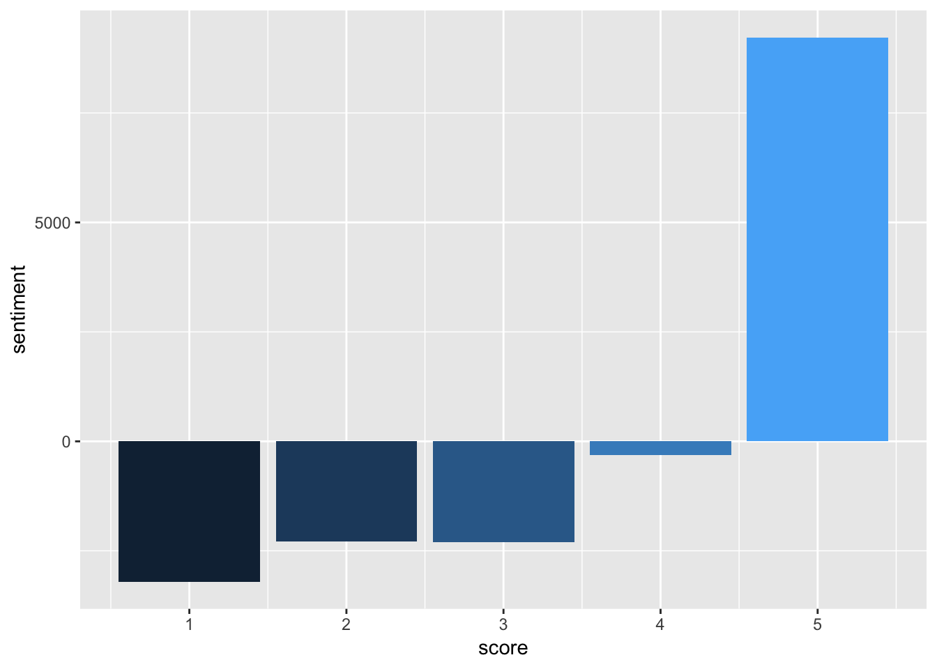
8 Closer Look at Lexicons
# there are more negative words in the nrc lexicon
get_sentiments("nrc") %>%
  filter(sentiment %in% c("positive", "negative")) %>%
  count(sentiment)
# also in nrc
get_sentiments("bing") %>%
count(sentiment)# the most common positive and negative words in all the reviews.
countBing = tidyData %>%
inner_join(get_sentiments("bing")) %>%
count(word, sentiment,sort = TRUE) %>%
ungroup()## Joining, by = "word"countBing9 Plotting Words
Plotting the negative and positive words
countBing %>%
  group_by(sentiment) %>%
  top_n(10) %>%
  ungroup() %>%
  mutate(word = reorder(word, n)) %>%
  ggplot(aes(word, n, fill = sentiment)) +
  geom_col(show.legend = FALSE) +
  facet_wrap(~sentiment, scales = "free_y") +
  labs(y = "Contribution to sentiment",
       x = NULL) +
  coord_flip()
## Selecting by n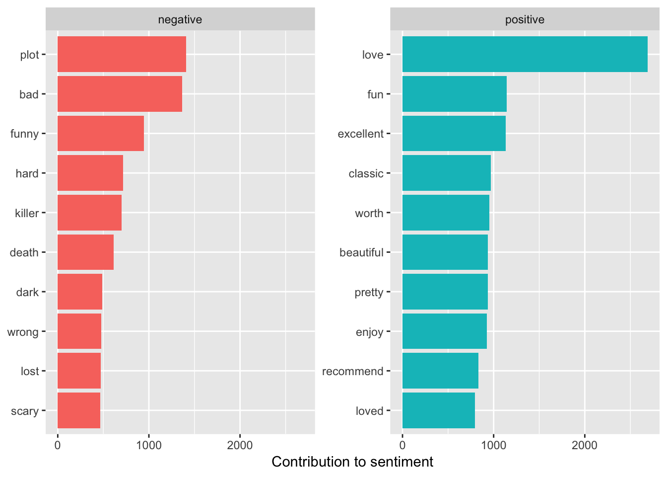
# we see some interesting classifications plot is probably not negative in the case
# of movie reviews...

# it might not be a good lexicon for reviews afterall
10 Removing Words
removing words that shouldnt be called negative or positive
# this is how we can make our own stop word library!!! super cool

custom_stop_words = bind_rows(data_frame(word = c("plot","br"),
                                          lexicon = c("custom")),
                               stop_words)

# we can remove br in this fashion


custom_stop_words
11 Word Cloud
Word cloud for top 100 words in all our 111,111 reviews.
if (!require("wordcloud")) install.packages("wordcloud")
library(wordcloud)

tidyData %>%
  anti_join(custom_stop_words) %>%
  count(word) %>%
  with(wordcloud(word, n, max.words = 100))
## Joining, by = "word"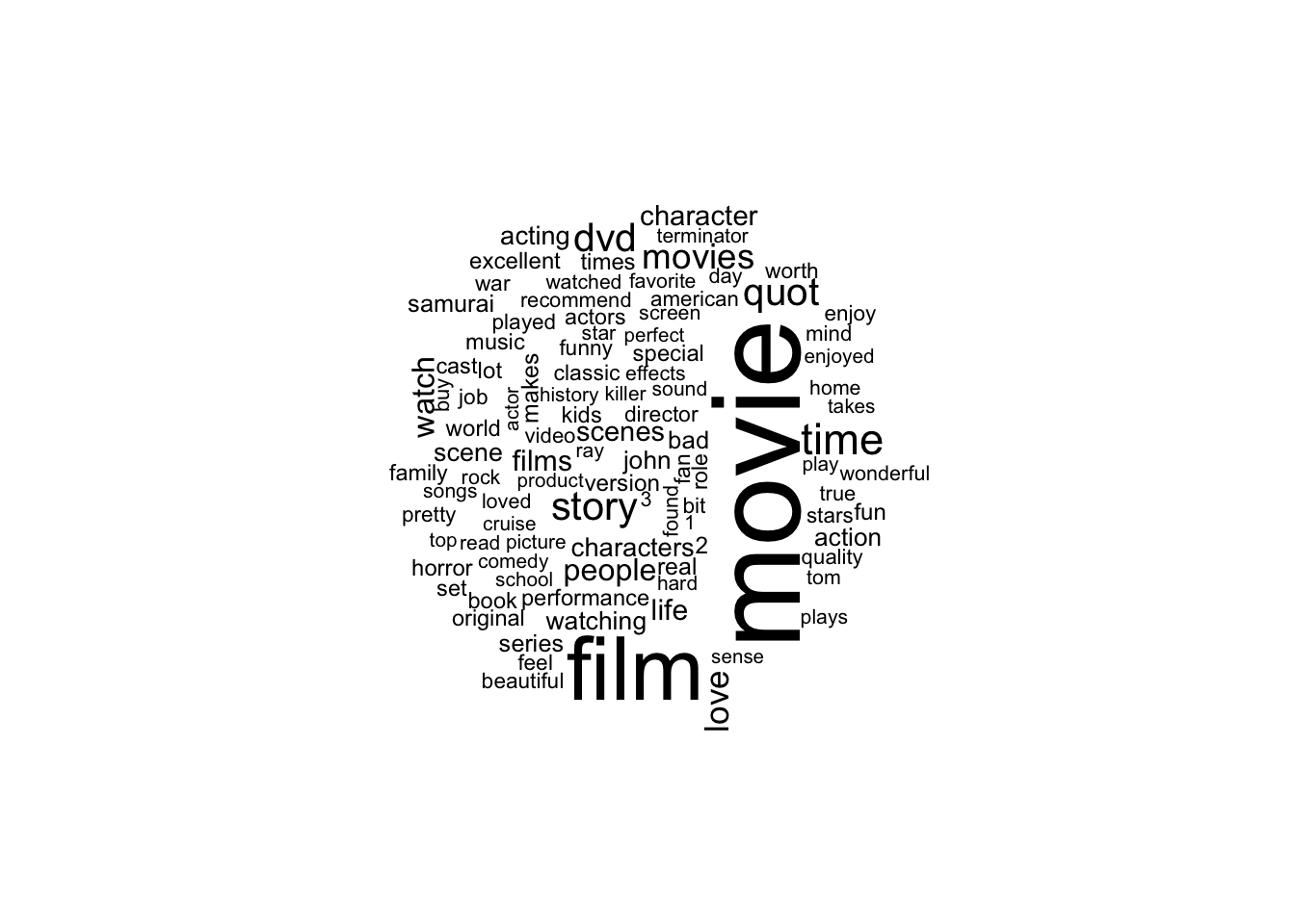
12 Word Cloud 2
Using a different word cloud library.
if (!require("reshape2")) install.packages("reshape2")

library(reshape2)

tidyData %>%
  anti_join(custom_stop_words) %>%
  inner_join(get_sentiments("bing")) %>%
  count(word, sentiment, sort = TRUE) %>%
  acast(word ~ sentiment, value.var = "n", fill=0) %>%
  comparison.cloud(colors = c("blue", "red"),
                   max.words = 100)
## Joining, by = "word"
## Joining, by = "word"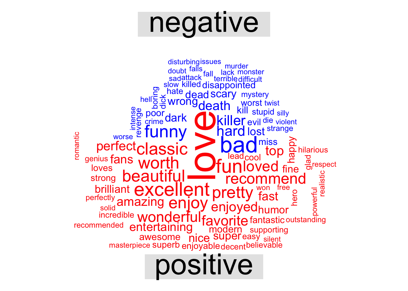
13 Ngrams
# this results in 85,326 "sentences" not sure how its less than the number of reviews...
tidySentences = data_frame(text = commentData$text) %>%
  unnest_tokens(sentence, text, token= "sentences")

tidySentences$sentence[2]
## [1] "investigative reporter karina danes (minnie driver) arrives from los angeles to pursue the story and angers both the local police and the factory owners who employee the undocumented aliens with her pointed questions and relentless quest for the truth.<br /><br />her story goes nationwide when a young girl named mariela (ana claudia talancon) survives a vicious attack and walks out of the desert crediting the blessed virgin for her rescue."bingnegative = get_sentiments("bing") %>%
filter(sentiment == "negative")
# words in each review
wordcounts = tidyData %>%
group_by(index, score) %>%
summarize(words = n())
# show the negative words ration of each review
tidyData1 = tidyData %>%
semi_join(bingnegative) %>%
group_by(index, score) %>%
summarize(negativewords = n()) %>%
left_join(wordcounts, by = c("index", "score")) %>%
mutate(ratio = negativewords/words) %>%
filter(index != 0) %>%
top_n(1) %>%
ungroup()## Joining, by = "word"## Selecting by ratio14 Song Lyric Analysis
if (!require("geniusR")) install.packages("geniusR")
library(geniusR)
if (!require("tidyverse")) install.packages("tidyverse")
library(tidyverse)
swift = genius_album(artist = "Taylor Swift", album = "Reputation")## Joining, by = c("track_title", "track_n", "track_url")riri = genius_album(artist = "Rihanna", album = "Anti")## Joining, by = c("track_title", "track_n", "track_url")library(tidytext)
tidy_swift = swift %>%
unnest_tokens(word, lyric) %>%
anti_join(stop_words) %>%
count(word, sort = TRUE)## Joining, by = "word"tidy_riri = riri %>%
unnest_tokens(word, lyric) %>%
anti_join(stop_words) %>%
count(word, sort = TRUE)## Joining, by = "word"tidy_swift = tidy_swift %>%
rename(swift_n = n) %>%
mutate(swift_prop = swift_n/sum(swift_n))
tidy_riri = tidy_riri %>%
rename(riri_n = n) %>%
mutate(riri_prop = riri_n/sum(riri_n))compare_words = tidy_swift %>%
full_join(tidy_riri, by = "word")
summary(compare_words)## word swift_n swift_prop riri_n
## Length:971 Min. : 1.000 Min. :0.00047 Min. : 1.000
## Class :character 1st Qu.: 1.000 1st Qu.:0.00047 1st Qu.: 1.000
## Mode :character Median : 1.000 Median :0.00047 Median : 1.000
## Mean : 3.208 Mean :0.00152 Mean : 3.446
## 3rd Qu.: 3.000 3rd Qu.:0.00142 3rd Qu.: 3.000
## Max. :81.000 Max. :0.03826 Max. :186.000
## NA's :311 NA's :311 NA's :532
## riri_prop
## Min. :0.0007
## 1st Qu.:0.0007
## Median :0.0007
## Mean :0.0023
## 3rd Qu.:0.0020
## Max. :0.1229
## NA's :532ggplot(compare_words, aes(swift_prop, riri_prop)) +
geom_abline() +
geom_text(aes(label=word), check_overlap = TRUE, vjust=1.5) +
labs(y="Rihanna", x="Taylor Swift") + theme_classic()## Warning: Removed 843 rows containing missing values (geom_text).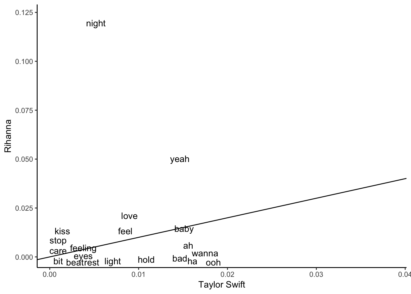
15 Over Time
if (!require("rvest")) install.packages("rvest")
library(rvest)
riridisc = 'https://en.wikipedia.org/wiki/Rihanna_discography'

disc <- riridisc %>%
  read_html() %>%
  html_nodes(xpath = '//*[@id="mw-content-text"]/div/table[2]') %>%
  html_table(fill = TRUE)


ririAlbums = disc[[1]]
TS_albums <- ririAlbums[2:9,1:2] %>%
separate(`Album details`, c("Released","Month","Day","Year"),
extra='drop') %>%
select(c("Title","Year"))
TS_albums$Year<-as.numeric(TS_albums$Year)riri_lyrics = TS_albums %>%
mutate(tracks = map2("Rihanna", Title, genius_album))## Joining, by = c("track_title", "track_n", "track_url")
## Joining, by = c("track_title", "track_n", "track_url")
## Joining, by = c("track_title", "track_n", "track_url")
## Joining, by = c("track_title", "track_n", "track_url")
## Joining, by = c("track_title", "track_n", "track_url")
## Joining, by = c("track_title", "track_n", "track_url")
## Joining, by = c("track_title", "track_n", "track_url")
## Joining, by = c("track_title", "track_n", "track_url")riri_lyrics = riri_lyrics %>%
unnest(tracks)library(tidytext)
tidy_riri <- riri_lyrics %>%
unnest_tokens(word, lyric) %>%
anti_join(stop_words, by = "word")tidy_riri %>%
count(word, sort=TRUE)words_by_year <- tidy_riri %>%
count(Year, word) %>%
group_by(Year) %>%
mutate(time_total = sum(n)) %>%
group_by(word) %>%
mutate(word_total = sum(n)) %>%
ungroup() %>%
rename(count = n) %>%
filter(word_total > 50)
nested_words <- words_by_year %>%
nest(-word)Copyright © 2019 Tomas Leriche. All rights reserved.